Remapping decisions

This document records the design rationale behind the significant technical choices in the remapping process that is applied to create all datasets¹. It is intended as a reference for contributors, reviewers, and downstream consumers of the produced HEALPix pyramids.

Why HEALPix?¶

HEALPix (Hierarchical Equal Area isoLatitude Pixelisation) tiles the sphere into pixels of exactly equal area at every resolution level. Originally developed for mapping the cosmic microwave background, it turns out to be exactly what analysis-ready climate data needs.

Area-weighted statistics are trivial¶

Every pixel covers the same solid angle, so a global mean is just the arithmetic mean of all pixels. No latitude-dependent cosine weighting is needed, and an entire class of subtle statistics bugs, forgotten or misapplied area weights, simply cannot occur.

Fields with missing values

This holds for complete fields. For fields with NaNs (ocean-only variables, sea ice, observation gaps), a coarse cell can be partly valid, and its value is the mean over that valid part only. Averages over coarse levels then need the valid fraction of each cell as a weight;

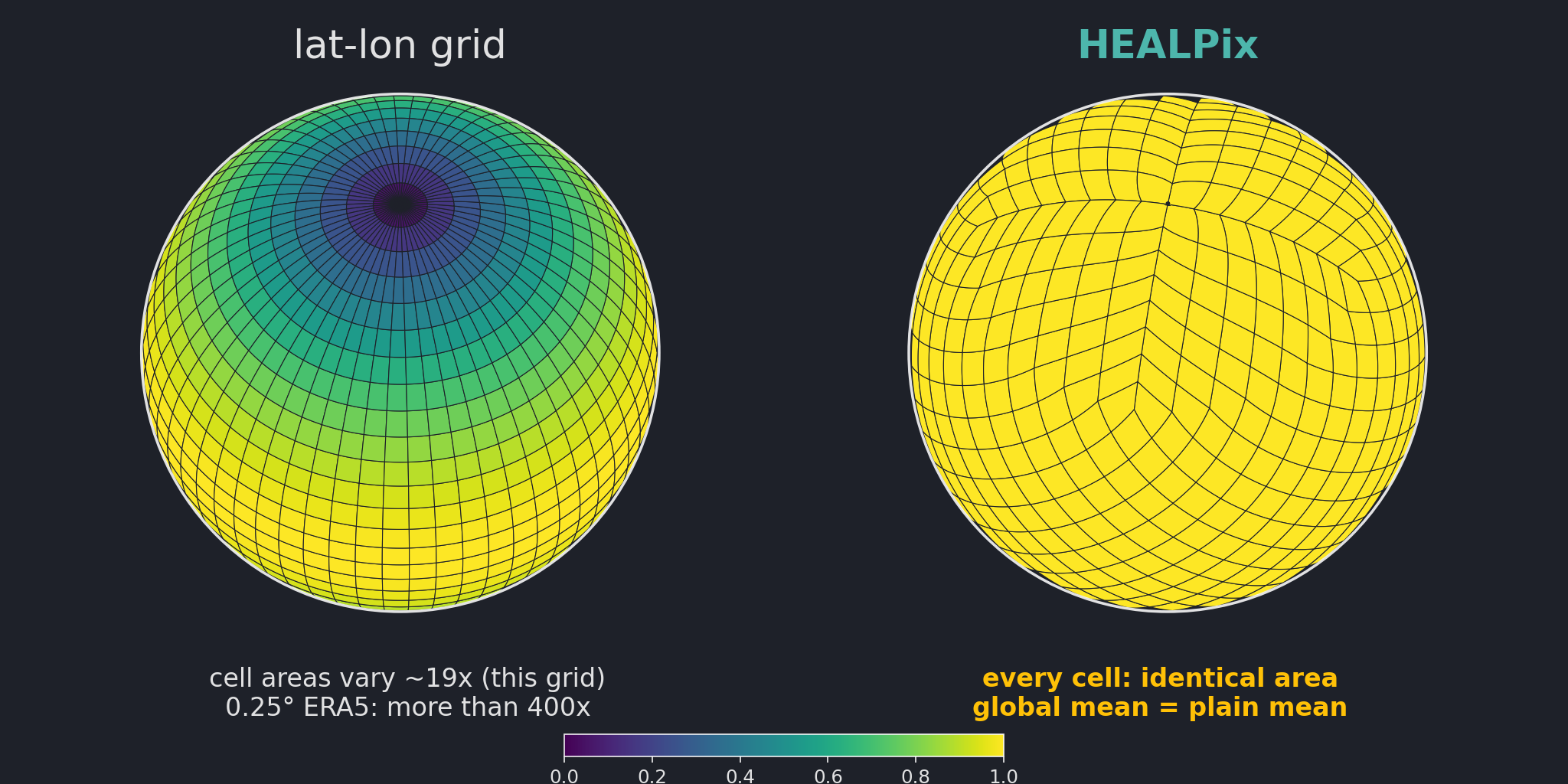
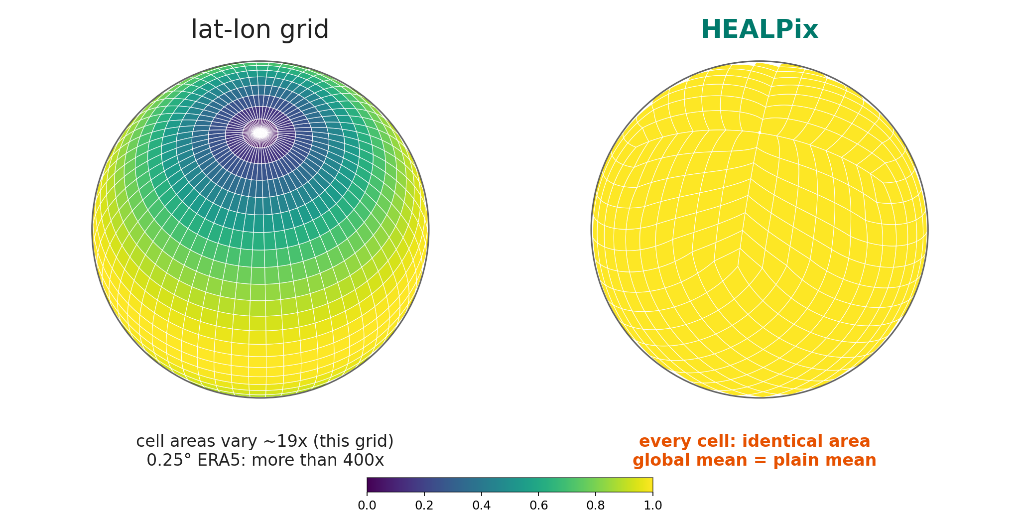
Equal area comparison — Cells coloured by their relative area. On a lat-lon grid (left), cell areas shrink with latitude; on a comparable 0.25° grid the largest cell is more than 400 times bigger than the smallest. On HEALPix (right), every cell is identical by construction.

No singularities at the poles¶

Regular lat-lon grids have converging meridians and vanishing cell areas at the poles, which force special-case handling in numerics, storage, and visualisation. HEALPix cells run right through the pole without anything special happening there.

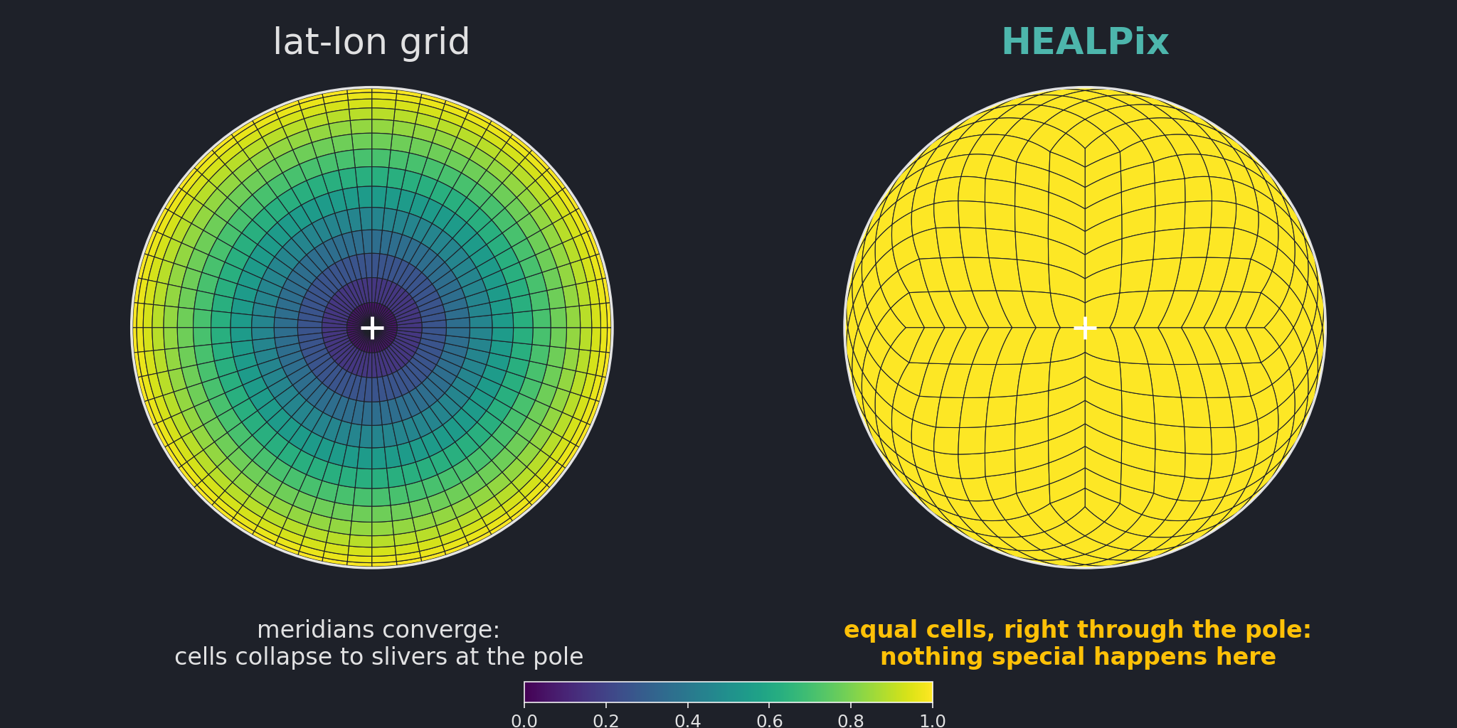
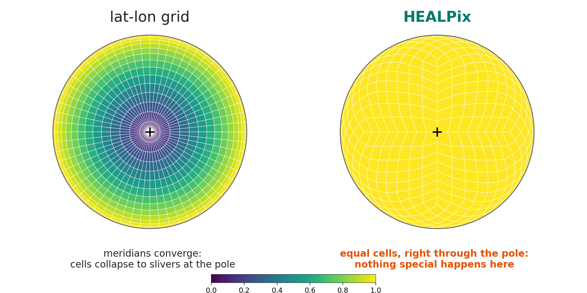
Pole view — Both grids viewed from directly above the North Pole (cross marks the pole). The lat-lon cells collapse into slivers at the centre; the HEALPix tessellation is unremarkable there, which is the point.

Nested ordering¶

HEALPix defines two pixel numbering schemes: ring ordering (pixels numbered along iso-latitude rings) and nested ordering (pixels numbered by a hierarchical quad-tree). The remapping procedure¹ defaults to nested ordering because it makes coarsening free.

In nested ordering, a parent pixel at level \(L\) with index \(i\) has children \(4i\), \(4i+1\), \(4i+2\), \(4i+3\) at level \(L+1\). Coarsening the full grid therefore reduces to reshaping the data array from \((n_\text{cells},)\) to \((n_\text{cells} / 4,\; 4)\) and reducing along the last axis, requiring no index lookup, no scatter, and no sorting.

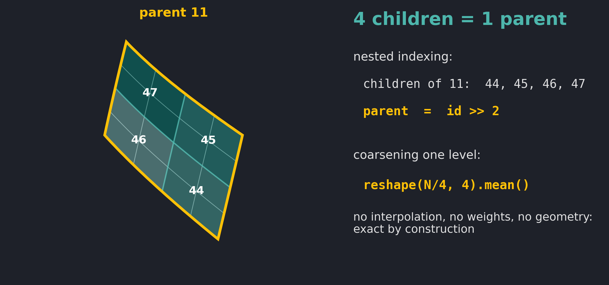
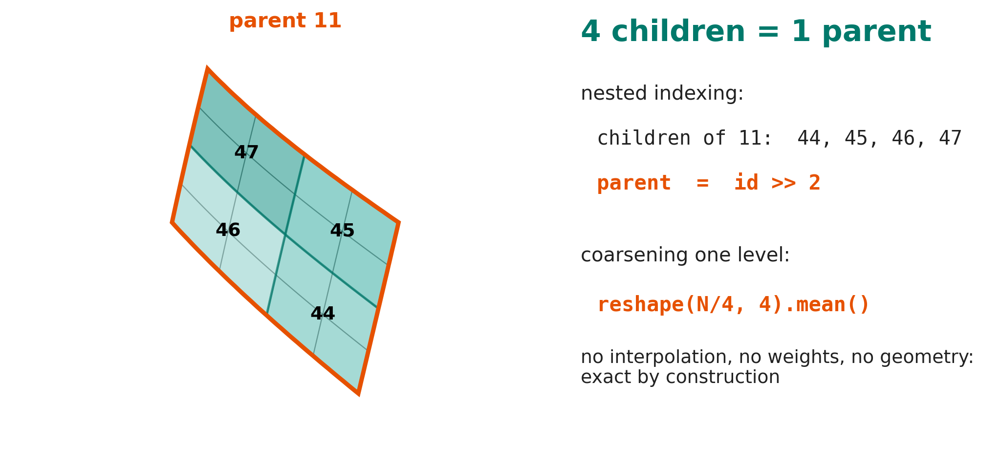
Nesting — A real level 2 cell (parent 11, amber) with its four level 3 children (44 to 47, teal) and sixteen level 4 grandchildren (thin outlines). The indices are the actual nested indices: children of parent p are 4p to *4p+3*.

HEALPix also supports ring ordering, but it does not have contiguous parent-child layout. Our remapping software¹ supports it, but in that mode every pyramid level is independently remapped from the source grid, which is substantially more expensive.

Sphere or ellipsoid¶

HEALPix can be defined on a perfect sphere, the original construction², or on the WGS84 ellipsoid⁷, where the cell boundaries are laid out in authalic latitude so that cells stay equal-area on the ellipsoid⁵⁸. grid-doctor uses the sphere by default.

Both definitions give the same results with ESMF, even though ESMF computes all overlap areas on the sphere⁶. healpix-geo returns the cell vertices of either definition in geodetic coordinates, the same coordinates the source data uses, so source and target mesh always share one coordinate space; the ellipsoidal definition only moves where the cell boundaries lie. The remaining distortion of the sphere approximation affects the numerator and denominator of every conservative weight³ almost equally and cancels to a relative error of about \(10^{-5}\) at level 10, smaller at finer levels.

What does not work is converting a remapped product from one definition to the other. Re-binning already averaged cells onto displaced cells adds a second interpolation step and roughly doubles the error. Products for either definition should always be remapped from the native data.

Route	Product	RMS error	× local contrast
A	native → spherical HEALPix	0.0840 K	0.94
B	native → ellipsoidal (WGS84) HEALPix	0.0841 K	0.94
C	A converted to ellipsoidal	0.1639 K	1.84

One day of MODIS-Aqua night-time SST (4 km) remapped to HEALPix level 10 (about 6.4 km) with ESMF conservative weights, about 2.66 million ocean cells. Each route is scored against a reference that bins the native pixels directly into cells of the same definition. The local contrast (median spread within groups of four neighbouring cells, 0.089 K) is the relevant scale because remapping errors live at the cell scale. A and B agree within 1 % between 60° S and 45° N and within 5 % poleward of that.

Different definitions are different grids¶

Two datasets on HEALPix at the same level are not on the same grid unless they use the same definition. The same cell index denotes a different patch of the Earth under the two definitions, displaced by the difference between geodetic and authalic latitude⁴:

\[ \varphi - \xi \approx \tfrac{e^2}{3} \sin 2\varphi \quad (\text{max } 7.7' \approx 14\ \mathrm{km\ at}\ 45°), \]

with WGS84 eccentricity \(e^2 \approx 0.006694\). That is about 2 cell widths at level 10, 9 at level 12 and 18 at level 13; at level 10, 99.8 % of all cells have a different index under the two definitions.

Data on different definitions must therefore not be compared, overlaid or differenced cell by cell, and cells must not be located with the other definition (for example lonlat_to_healpix with a different ellipsoid than the data was produced with). Otherwise the field appears shifted by up to 14 km: fronts, coastlines and swath edges land in the wrong cells. To compare such datasets, remap both from their native data onto the same definition.

Target level selection¶

The target HEALPix level for each source dataset is chosen as the highest level whose characteristic pixel spacing is coarser than or comparable to the source resolution. The heuristic is:

\[ \ell = \left\lfloor \log_2 \frac{58.6°}{\Delta} \right\rfloor \]

where \(\Delta\) is the estimated source grid spacing in degrees. The constant 58.6° is the approximate pixel spacing at level 0, derived from \(360° \;/\; \sqrt{12 \times 4^0}\).

This ensures that the HEALPix grid does not oversample the source. Lower pyramid levels are derived by coarsening, not by remapping, so no additional information is fabricated.

Level	nside	Pixels	Approx. spacing
0	1	12	58.6°
3	8	768	7.3°
5	32	12 288	1.8°
7	128	196 608	27.5′
9	512	3 145 728	6.9′
10	1024	12 582 912	3.4′

Remapping methods¶

Remapping is performed by ESMF, which computes the geometric overlap between source and target cells and produces a sparse weight matrix that is applied to the data. The remapping software supports two remapping methods, chosen by variable type.

Conservative remapping (continuous fields)¶

Used for temperature, precipitation, radiation, wind, and all other fields that represent continuous physical quantities.

Conservative remapping computes area-weighted averages: each weight is proportional to the fractional overlap area between a source cell and a target cell. The key property is integral preservation, the area-integral of the field over any target cell equals the sum of the area-integrals of the contributing source cells.

This is the only method that correctly handles sub-pixel variability. If a HEALPix cell straddles a strong SST gradient, the conservative average reflects the true area-weighted mean rather than the value at a single sampled point.

Nearest-neighbour remapping (categorical fields)¶

Used for land-sea masks, land cover classes, soil type, and all other fields where values are discrete labels.

Nearest-neighbour assigns each target cell the value of the closest source cell centre. This guarantees that the output contains only values that actually exist in the source, no interpolated intermediate classes like "land-use 3.7" can appear.

Linear or bilinear interpolation is explicitly not supported. While it can produce smoother-looking fields, it fabricates values that were not present in the original data.

Weight generation¶

Remapping weights are precomputed and stored as reusable NetCDF files. Weight generation is the most expensive step in the pipeline, but it only needs to happen once per combination of source grid and target HEALPix level. Subsequent runs reuse the cached weight file.

For moderate grids, weights are generated in memory using ESMF's Python bindings (ESMPy). For very large grids where this would exceed available RAM, grid-doctor¹ writes both meshes to temporary files and invokes the standalone ESMF_RegridWeightGen command under MPI, with a configurable number of ranks.

Grid-doctor¹ automatically classifies the source grid and constructs the appropriate mesh representation:

Source type	Examples	Detection
Regular	ERA5, CMIP on lat-lon grids	1-D `lat` and `lon` coordinates
Curvilinear	NEMO, WRF	2-D `lat(y, x)` and `lon(y, x)`
Unstructured	ICON, MPAS	Dimension named `cell` / `ncells`, or `CDI_grid_type` attribute

Every weight file is annotated with provenance metadata (grid_doctor_method, grid_doctor_level, grid_doctor_order, source grid details) so that downstream tools can verify how the weights were produced.

Weight application¶

Applying the weight matrix to data is a sparse matrix multiplication. The full batch of time steps is reshaped into a single dense matrix and multiplied in one operation, which is typically 10–50× faster than applying the weights one time step at a time. GPU acceleration (via CuPy) and JIT compilation (via Numba) are used automatically when those packages are installed. See Performance: application backends for details.

Missing-value handling during remapping¶

Source datasets commonly contain NaN values, for instance land pixels in an ocean dataset, gaps in satellite swaths, or masked regions. The missing_policy parameter controls how these are treated during weight application.

Renormalize (default)¶

Source cells that are NaN are excluded from the weighted sum. The weights of the remaining valid source cells are rescaled so they sum to 1. A target cell receives a valid value as long as at least one contributing source cell is valid.

This is the appropriate choice for virtually all climate fields. A HEALPix cell on a coastline that partly overlaps land (NaN) and partly ocean still receives a valid SST from the ocean fraction.

Propagate¶

If any contributing source cell is NaN, the target cell is set to NaN. No partial averages are computed.

This mode exists for strict budget-closure applications. If you are integrating total precipitation over a HEALPix cell and one source cell is missing, the renormalized average looks valid but represents a biased estimate over a subset of the area. For budget-closure studies it is preferable to have a NaN than a plausible-looking number derived from incomplete coverage.

Note that this mode is very aggressive: a single NaN source cell at the edge of a target cell's footprint is enough to discard it. Along coastlines, swath edges, and orbit gaps, large portions of the output will be NaN.

Point binning (swath and station data)¶

Gridded datasets are remapped with ESMF as described above. Point-sampled data — satellite Level-2 swaths, station records, trajectories — cannot use that path for two structural reasons: every granule has unique geometry, so the precomputed weight matrix can never be reused, and ESMF's nearest source-to-destination method assigns a value to every destination cell, which would smear a narrow swath over the entire globe.

Point data is therefore binned: each sample is assigned to the HEALPix cell containing its coordinates and all samples per cell are reduced. The available reductions mirror the two remapping methods:

Mean binning (continuous fields). In the oversampled limit — sample spacing much finer than the target cell spacing — the per-cell sample mean converges to the area-weighted mean, making it a first-order approximation of conservative remapping. This validity condition is enforced by choosing the target level from the sample spacing with the same heuristic used for gridded data; a swath is never binned into cells finer than its own pixel spacing.
Mode binning (categorical fields). The most frequent class per cell, the binning analogue of nearest-neighbour remapping. Ties are broken deterministically towards the lowest class value. As with nearest-neighbour remapping, no interpolated intermediate classes can appear.
min / max / count are available for extrema and coverage diagnostics.

A per-sample sum is deliberately not offered: it scales with sample density (orbit overlap, across-track pixel count) rather than any physical integral, and therefore violates the integral-preservation rationale that motivates conservative remapping. Root-mean-square reductions are likewise excluded because they do not commute with mean coarsening in the pyramid; if an RMS quantity is required, bin the squared field with the mean and apply the square root at read time.

Sphere, also for satellite data¶

Satellite geolocation is geodetic (WGS84). Binning indexes cells on the perfect sphere, like remapping, by assigning each geodetic position to the cell that contains it; this is as accurate as binning on the ellipsoid (see Sphere or ellipsoid). Data binned on one definition is not comparable cell by cell with data on the other: the cells are displaced by up to ~0.13° (~14 km) at 45° latitude, several to dozens of pixels at typical swath target levels.

Minimum sample count and coverage tracking¶

A cell is set to NaN when it receives fewer than min_count valid samples (default: 1). Optionally, a companion <variable>_count variable records the number of valid samples per cell. Publishing the count is recommended: it makes coverage auditable, enables unbiased count-weighted merging of overlapping granules, and is the point-data analogue of a valid-area fraction for coarsened grids.

Pyramids from binned data¶

Binned datasets carry the full standard metadata (crs variable, healpix_* and grid_doctor_* attributes) and dense cell layout, so pyramid construction reuses the ordinary coarsening machinery unchanged, including the 50% minimum-valid-fraction rule. The recorded method (grid_doctor_method = "binned-mean" or "binned-mode") drives the automatic mean-vs-mode coarsening selection, just as "conservative" and "nearest" do for remapped data.

Pyramid construction and coarsening¶

The multi-resolution pyramid is built by first remapping the source dataset to the finest HEALPix level, then deriving all coarser levels by iterated coarsening, one level at a time, always a factor of 4. Every level builds on the previous one, so the whole pyramid is a single lazy computation (see Chunked application and single-pass writes).

Why coarsen rather than remap at each level?¶

Remapping from the original source grid at every level would be correct but wasteful: each level would require a separate weight file, and weight generation cost scales with the product of source and target cell counts. Coarsening is essentially free, a reshape plus a vectorised reduction, and produces identical results for nested HEALPix grids because the nested pixel hierarchy exactly matches the coarsening hierarchy.

Mean coarsening (continuous fields)¶

For continuous fields (those remapped with conservative weights), each coarse cell's value is the mean over all valid finest-level cells beneath it. This is not the same as the mean of its 4 children once children are only partly valid: a child built from a single valid finest-level cell would otherwise count as much as a child built from four. Repeated over several levels, that mean of means drifts away from the finest level.

The pyramid therefore carries two running totals per cell instead of a mean: the sum of the valid finest-level values and their count. Both coarsen exactly by summing groups of 4, and the mean is only formed when a level is written:

\[ \bar{x}_\text{parent} = \frac{\sum_{c} s_c}{\sum_{c} n_c}, \qquad s_c = \sum_{\text{valid } i \in c} x_i, \quad n_c = \#\{\text{valid } i \in c\} \]

Every level is therefore identical to coarsening directly from the finest level, while each step stays a local reduction of 4 neighbouring cells.

Mode coarsening (categorical fields)¶

For categorical fields (those remapped with nearest-neighbour weights), averaging class labels is meaningless. Instead, each parent cell receives the mode (most frequent value) of its valid children. Ties are broken by the first occurrence.

The coarsening mode is inferred automatically from the remapping method stored in the dataset attributes: grid_doctor_method = "nearest" triggers mode coarsening, "conservative" triggers mean coarsening. An explicit coarsen_mode parameter is available to override this.

Unlike the mean, a mode of modes is not the mode of all finest-level cells, and mode coarsening is applied level by level, with the minimum valid fraction checked against the 4 children at each step.

Minimum valid fraction (default: 50%)¶

For mean coarsening, a cell is set to NaN when fewer than half of the finest-level cells beneath it are valid. The threshold is applied to this cumulative fraction, not to the 4 children of each step.

Representativeness. A cell's value should represent the majority of its area. Because the threshold uses the finest-level count, the value is guaranteed to cover at least half of the cell's area at every level. A per-step rule could not guarantee this: 2 valid children out of 4, each built from 2 valid children out of 4, cover only a quarter of the area two levels up. Below the threshold, a few pixels' values would "speak for" an area that has no data, which is indistinguishable from interpolation into unknown territory.

Cells masked by the threshold keep their running sums and counts, so their valid data still contributes to coarser levels where it is part of a majority.

Cascade prevention. Each coarsening step is a factor-of-4 reduction. If only 1 of 4 valid children were sufficient, a single valid pixel at the finest level could survive every coarsening step: 1/4 at level \(N-1\), that surviving parent is again 1/4 at level \(N-2\), and so on. After \(k\) steps it represents a fraction of \(4^{-k}\) of the area it claims to cover. This is the "Siberian lake problem" observed with MODIS SST: a single lake pixel at level 10 bled through 7 coarsening steps to level 3, covering a 16 384× larger area. With a 50% threshold, the cascade is impossible, the pixel is discarded at the very first step because 1/4 < 1/2. A feature can only survive coarsening if it covers at least half the area at every scale, which is exactly when it is a real, resolvable feature at that resolution.

The threshold is configurable with min_valid_fraction. Set it to 0 to keep every cell that contains any valid data, for instance when the coarse levels are only used for weighted aggregates.

Averaging over coarse levels: valid fractions¶

Because every coarse value is a mean over its valid area, a plain mean over coarse cells weights a coastal cell that is 10% ocean as much as an open-ocean cell. The level-to-level consistency of the pyramid only holds for means weighted by the number of valid finest-level cells: with two coarse cells, one fully valid at 10 °C (4 valid cells) and one with a single valid cell at 20 °C, the finest-level mean is (4 × 10 + 20) / 5 = 12 °C, while the plain mean of the two coarse values is 15 °C. Both coarse values are correct; the plain average is not.

The weights cannot be folded into the stored values without losing their meaning (a coastal cell would no longer hold the SST of its ocean part). Instead, the pyramid can store them alongside:

pyramid = gd.create_healpix_pyramid(ds, valid_fraction=True)

adds <name>_valid_fraction (float32, fraction of valid finest-level cells, linked through the CF ancillary_variables attribute) to every level, including the finest one. Global or regional means then agree across all levels:

ds = pyramid[3]
ds.sst.weighted(ds.sst_valid_fraction.fillna(0)).mean("cell")

The option is opt-in because the fraction has the shape of its variable:

True stores a fraction for every cell variable, with its full shape. This is correct for masks that change over time or height (sea ice, clouds, orography on pressure levels).
"static" stores a single cell-only fraction taken from the first time step / level. It is tiny, but only correct when the mask never changes, as for a land-sea mask.
A list of names, or a mapping such as {"sst": "static", "ice": True}, restricts the fractions to selected variables.

Fractions are mostly exactly 0 or 1 and compress well; in a test with 8 time steps the full-shape fractions added about 7% to the store, the static ones under 1%. This mirrors the ocean_fraction variables of the nextGEMS HEALPix output.

Output metadata and CRS convention¶

Every output dataset carries a standardised set of metadata.

Global attributes¶

Attribute	Description
`healpix_level`	HEALPix refinement level
`healpix_nside`	\(2^\ell\)
`healpix_order`	`nested` or `ring`
`grid_doctor_version`	Package version that produced the data
`grid_doctor_method`	`conservative` or `nearest`
`grid_doctor_coarsened_from_level`	Level the values were coarsened from: the finest level for pyramids, the input level for `coarsen_healpix` (coarsened levels only)
`grid_doctor_coarsen_mode`	`mean` or `mode` (coarsened levels only)
`grid_doctor_min_valid_fraction`	Threshold below which cells were set to NaN: cumulative over finest-level cells for `mean`, per coarsening step for `mode` (coarsened levels only)

CRS variable¶

A scalar coordinate variable named crs follows the CF grid_mapping convention. It carries attributes that describe the coordinate reference system:

crs: float64
    grid_mapping_name: healpix
    healpix_nside: 1024
    healpix_level: 10
    healpix_order: nested

Every spatially-dimensioned data variable carries grid_mapping = "crs" so that CF-aware tools can discover the projection automatically. This convention is validated against the gridlook viewer, which uses grid_mapping_name == "healpix" to detect and render HEALPix datasets.

Storage format¶

Pyramids are written as Zarr v2 stores with consolidated metadata, one store per level (level_0.zarr, level_1.zarr, …). Zarr v2 is used because ecosystem support for v3 is still maturing: client libraries such as zarr-python, zarr-js (used by gridlook and similar web viewers), xarray, and zarrita have stable, well-tested v2 implementations, while v3 support varies in completeness. The transition to v3 is planned once the client ecosystem has converged.

Zarr's chunked, cloud-native layout enables byte-range reads from S3 without downloading entire files, which is essential for interactive visualisation where only a single chunk of a single variable at a single level needs to be fetched.

High-level regional datasets: implicit coordinates¶

Small-area datasets at very high levels (16 and beyond) keep the dense global convention — cell position equals cell index — but stop materialising what the index already implies. Above level 10 (WRITE_COORDS_MAX_LEVEL), stores are written without cell/latitude/longitude coordinate arrays: at level 16 those two float64 arrays would cost ~800 GB while the regional payload is megabytes, and unlike the data variables they are never fill values, so empty-chunk elision cannot help. Such stores carry grid_doctor_implicit_coords = 1, retain the crs variable and all healpix_* attributes, and remain byte-identical in layout to an ordinary dense store.

Access is region-driven through range selection. Nested ordering guarantees that every coarse-level parent corresponds to one contiguous fine-level index range, so a bounding-box query decomposes into a handful of contiguous reads that align one-to-one with power-of-four chunks. Coordinates are reconstructed on the fly for exactly the cells returned. Combined with fill_value = NaN and empty-chunk elision on the data variables, storage and access cost are proportional to the domain, not the globe, while cross-dataset and cross-level alignment stay a bit-shift (parent = id >> 2k) exactly as for every other nested HEALPix dataset.

Levels at or below the threshold within the same pyramid are written with materialised coordinates as usual, so coarse overview levels stay directly consumable by CF-aware viewers.

Performance: application backends¶

The sparse weight-matrix multiplication supports three backends, selected automatically based on what is installed.

Batched SciPy (always available) reshapes all time steps into a single dense matrix and performs one sparse matmul, delegating to BLAS for the dense side. This is typically 10–50× faster than per-slice application.

Numba (optional) JIT-compiles a fused kernel that computes the weighted sum, NaN mask, and renormalization in a single pass over the sparse matrix structure. This halves memory traffic for single-slice workloads.

CuPy (optional) transfers the weight matrix to the GPU once and applies it via cuSPARSE. This is worthwhile for large target grids (HEALPix level 10+) with many time steps, where the transfer cost is amortised over the batch.

The backend can be overridden explicitly via backend="scipy", "numba", or "cupy" in any remapping call.

Chunked application and single-pass writes¶

For dask-backed input, the regridded field is chunked along cell (cell_chunks, by default 4^10 cells). Rows of the weight matrix are independent, so each output chunk is computed from its own block of matrix rows; the blocks share the matrix memory instead of copying it. No task holds the whole HEALPix field, and the coarser levels keep the same chunking because every coarsening step only combines groups of 4 neighbouring cells.

Inside dask tasks the Numba kernels run single-threaded: dask already runs many tasks in parallel, and a multi-threaded kernel per task would start one thread team per task and exhaust the process thread limit on many-core nodes. Without dask, the multi-threaded kernels are used.

save_pyramid writes all levels in a single computation, so the regridding of each finest-level chunk runs exactly once and is shared by all coarser levels. Computing levels separately (for example pyramid[5].compute() followed by pyramid[4].compute()) regrids the source again each time; persist() the finest level when exploring interactively.

References¶

Remapping is realised with a uniform remapping software grid-doctor ↩↩↩↩↩
Górski, K. M., et al. (2005). HEALPix: A Framework for High-Resolution Discretization and Fast Analysis of Data Distributed on the Sphere. The Astrophysical Journal, 622(2), 759–771. https://doi.org/10.1086/427976 ↩
Jones, P. W. (1999). First- and Second-Order Conservative Remapping Schemes for Grids in Spherical Coordinates. Monthly Weather Review, 127(9), 2204–2210. https://doi.org/10.1175/1520-0493(1999)127%3C2204:FASOCR%3E2.0.CO;2 ↩
Snyder, J. P. (1987). Map Projections: A Working Manual. U.S. Geological Survey Professional Paper 1395. Auxiliary latitudes (authalic, geocentric) and radii of curvature: Ch. 3. https://doi.org/10.3133/pp1395 ↩
Gibb, R. G. (2016). The rHEALPix Discrete Global Grid System. IOP Conference Series: Earth and Environmental Science, 34, 012012. https://doi.org/10.1088/1755-1315/34/1/012012 ↩
ESMF Reference Manual, Regridding: conservative methods operate on the surface of the sphere with great-circle cell edges. https://earthsystemmodeling.org/docs/release/latest/ESMF_refdoc/ ↩
NGA (2014). Department of Defense World Geodetic System 1984 (NGA.STND.0036_1.0.0_WGS84). Defining parameters: \(a = 6378137\) m, \(1/f = 298.257223563\). ↩
healpix-geo, HEALPix for the geosciences, with WGS84 ellipsoid support via auxiliary latitudes. https://github.com/GRID4EARTH/healpix-geo, reference-system background: https://healpix-geo.readthedocs.io/en/stable/reference-system.html ↩