Cutting out a region
ds.sel(lat=slice(35, 70), lon=slice(-15, 35)) is the line everybody
reaches for first, and on a HEALPix store it raises. There is no lat
dimension to slice. There is one horizontal dimension, cell, and its index
encodes position in a way that a slice object knows nothing about.
There are two honest ways to cut out a box. The difference between them is the difference between an analysis that runs in a second and one that downloads the planet first.
The obvious way: mask on the coordinates
Global pyramid levels ship the cell centre coordinates with the store, so a boolean mask is immediate.
import cartopy.crs as ccrs
import matplotlib.pyplot as plt
import numpy as np
import xarray as xr
from healpix_geo import nested

URL = "s3://reanalysis/healpix/era5/P1M/level_7.zarr"
S3 = {"anon": True, "endpoint_url": "https://s3.waterpark.dkrz.de"}

ds = xr.open_zarr(URL, storage_options=S3, chunks=None)
level = ds.attrs["healpix_level"]
field = ds["tas"].sel(time="2021-07").squeeze()

LON_MIN, LON_MAX = -15.0, 35.0
LAT_MIN, LAT_MAX = 35.0, 70.0

# Coordinates come out of the store in 0..360. A box that crosses the prime
# meridian, which most European boxes do, needs them in -180..180 first.
# This is the most common reason a region comes back empty.
longitude = ds["longitude"].values
longitude = np.where(longitude > 180.0, longitude - 360.0, longitude)
latitude = ds["latitude"].values

inside = (
    (longitude >= LON_MIN) & (longitude <= LON_MAX)
    & (latitude >= LAT_MIN) & (latitude <= LAT_MAX)
)
masked = field.isel(cell=np.flatnonzero(inside))

print(f"{masked.sizes['cell']} of {field.sizes['cell']} cells inside the box")
print(f"regional mean {float(masked.mean()):.2f} K")
Note what the mean did not need: no weights. The cells are equal area, so the arithmetic mean over an arbitrary subset of them is already the area weighted mean over whatever shape that subset makes.
What the obvious way costs
The mask is computed from coordinates, which means it needs the coordinates, which means it needs the store's full cell axis even though the answer is a few per cent of it.
print(f"read to build the mask: {field.nbytes / 1e6:.1f} MB")
print(f"actually wanted:        {masked.nbytes / 1e6:.2f} MB")
At level 7 that is a rounding error and the mask is the right answer. At level 12 it is a gigabyte to select a country, and at level 16 the coordinate arrays alone would be fifty billion entries, which is why the regional stores do not carry them at all.
The scalable way: ask HEALPix which cells the box covers
Invert the question. Instead of reading every cell and testing it, ask the grid which cell indices cover the box and read only those.
zone_coverage is the function for a longitude/latitude rectangle. It
takes the bounding box as (lon_min, lat_min, lon_max, lat_max) and
returns a superset of the cells inside it.
covering, _, fully_inside = nested.zone_coverage(
    (LON_MIN, LAT_MIN, LON_MAX, LAT_MAX), level
)
covering = np.sort(np.asarray(covering).astype("int64"))

print(f"{covering.size} cells cover the box, "
      f"{int(np.sum(fully_inside))} of them lie fully inside it")
Not every coverage function means a lon/lat rectangle
nested.box_coverage looks like it should do this job and does
something else. It takes a centre and half extents, and the box it
describes is bounded by great circles, which is not the same shape as
a lon/lat rectangle anywhere away from the equator. Handed this box's
numbers it returns a region reaching from 43 degrees west to 63 east,
and still misses cells in the corners. It is the right function for a
rotated footprint such as a satellite swath, and the wrong one here.
nested.cone_coverage is the circle, which is usually what you want
around a station or a city.
Cover, then trim
The coverage is a superset: it includes cells that overlap the boundary
without their centre being inside. The fully_covered flag is enough when
you want every cell touching the area, which is the right definition for a
budget or a mask.
When you want the centres, trim it. The point is that the coordinates are computed for the covered cells only, never for the global axis, so this step costs the same at level 16 as it does here.
cover_lon, cover_lat = nested.healpix_to_lonlat(covering.astype("uint64"), level)
cover_lon = np.asarray(cover_lon)
cover_lon = np.where(cover_lon > 180.0, cover_lon - 360.0, cover_lon)
cover_lat = np.asarray(cover_lat)

trimmed = covering[
    (cover_lon >= LON_MIN) & (cover_lon <= LON_MAX)
    & (cover_lat >= LAT_MIN) & (cover_lat <= LAT_MAX)
]

print(f"coordinates computed for {covering.size} cells, "
      f"{100 * covering.size / field.sizes['cell']:.1f}% of the grid")
print(f"trimmed to {trimmed.size} cells; the mask found {masked.sizes['cell']}")
assert set(trimmed.tolist()) == set(np.flatnonzero(inside).tolist())
Identical answers, by two routes that scale very differently.
Why the reads are cheap too
The indices are not scattered. In nested ordering, cells near each other on the sphere are near each other in the index, so a compact region resolves into a handful of contiguous runs, and each run is one byte range rather than a shopping list.
runs = np.flatnonzero(np.diff(covering) != 1).size + 1
print(f"{covering.size} indices form {runs} contiguous runs")
print(f"that is {runs} range requests, not {covering.size}")

selected = field.isel(cell=covering)
The plot
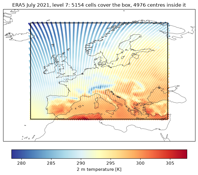
Drawn as cell centres rather than a raster, because at this point the cells are the subject. At level 7 they are about 50 km across, so they tile the box densely enough to read as a map. The cells outside the outline are the coverage's margin, which the trim removes.
fig, ax = plt.subplots(
    figsize=(9, 6.8), subplot_kw={"projection": ccrs.PlateCarree()}
)
ax.coastlines(linewidth=0.5, color="0.2")
ax.set_extent([LON_MIN - 10, LON_MAX + 10, LAT_MIN - 8, LAT_MAX + 5],
              crs=ccrs.PlateCarree())

scatter = ax.scatter(
    cover_lon, cover_lat, c=selected.values, s=16, cmap="RdYlBu_r",
    edgecolor="none", transform=ccrs.PlateCarree(),
)
ax.plot(
    [LON_MIN, LON_MAX, LON_MAX, LON_MIN, LON_MIN],
    [LAT_MIN, LAT_MIN, LAT_MAX, LAT_MAX, LAT_MIN],
    color="black", lw=1.4, transform=ccrs.PlateCarree(),
)

fig.colorbar(scatter, ax=ax, orientation="horizontal", pad=0.05, shrink=0.8,
             label="2 m temperature [K]")
ax.set_title(
    f"ERA5 July 2021, level {level}: {covering.size} cells cover the box, "
    f"{trimmed.size} centres inside it", fontsize=11,
)

fig.savefig("03_region_bbox.png", dpi=110, bbox_inches="tight", facecolor="white")
Cutting out a region
Which one to use
Mask on coordinates up to about level 9, where the full cell axis is still a few million entries and the code is shorter. Above that, cover and trim, and select before you touch any data.
The regional data guide works the second pattern through in full for the city-scale stores at level 16 and above, where it is not an optimisation but the only thing that works, and where aligning the cover with the store's chunk size starts to pay as well.
Run it yourself: examples/03_region_bbox.py